Getting started
Welcome to the CensoredDistributions documentation! This section is designed to help you get started with the package. It includes a quickstart guide, frequently asked questions (FAQ) section, and tutorials that will help you get started with CensoredDistributions for specific tasks. See the sidebar for the list of topics.
Introduction
Delay distributions play a crucial role in various fields, including epidemiology, reliability analysis, and survival analysis. These distributions describe the time between two events of interest, such as the incubation period of a disease or the time to failure of a component. Accurately estimating and calculating these distributions is essential for understanding the underlying processes and making informed decisions.
The estimation of delay distributions often faces the following challenges:
- Primary event within interval censoring: The primary event (e.g., exposure to a pathogen or the start of a process) is often observed with some degree of interval censoring. This means that the exact time of the event is not known, but rather, it is known to have occurred within a certain time interval, commonly a day.
As a result, any distribution based on these primary events is a combination of the underlying true distribution and the censoring distribution.
- Truncation: The observation of delay distributions is often conditioned on the occurrence of the secondary event. This leads to a truncation of the observed distribution, as delays longer than the observation time are not captured in the data.
Consequently, the observed distribution is a combination of the underlying true distribution, the censoring distribution, and the observation time.
- Secondary event within interval censoring: The secondary event (e.g., symptom onset or the end of a process) is also frequently observed with within an interval.
This additional layer of censoring further complicates the estimation of the delay distribution.
- Double event within interval censoring Both the primary and secondary events are censored so that we know they occurred in an interval but not precisely when.
The CensoredDistributions.jl package aims to address these challenges by providing tools to manipulate primary censored delay distributions and to extend these distributions to account for both truncation and secondary event censoring. By accounting for the censoring and truncation present in the data, the package enables more accurate estimation and use of the underlying true distribution.
In this quickstart, we will provide a quick introduction to the main functions and concepts in the CensoredDistributions.jl package. We will cover the mathematical formulation of the problem, demonstrate the usage of the key functions, and provide signposting on how to learn more.
Packages used in this getting started guide
Loading the packages
# Import the package
using CensoredDistributions
using Distributions
using Random
using Plots

# Set the seed for reproducibility
Random.seed!(123)Random.TaskLocalRNG()Primary event censoring
The mathematical formulation for primary event censoring involves several key steps:
- Primary event times (
) are generated from a specified primary event distribution, in this case uniform between 0 and 1:
primary_event = Uniform(0, 1)Distributions.Uniform{Float64}(a=0.0, b=1.0)- Delays (
) are generated from a specified delay distribution, here a log-normal:
dist = LogNormal(1.5, 0.75)Distributions.LogNormal{Float64}(μ=1.5, σ=0.75)This corresponds to:
x = 0:0.01:15
plot(x, pdf.(dist, x))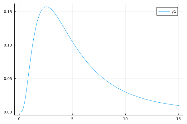
- Total delays (
) are calculated by adding the primary event times and delays:
Now we combine these two distributions to create a primary censored distribution:
prim_dist = primary_censored(dist, primary_event)CensoredDistributions.PrimaryCensored{Distributions.LogNormal{Float64}, Distributions.Uniform{Float64}, CensoredDistributions.AnalyticalSolver{Integrals.QuadGKJL{typeof(LinearAlgebra.norm), Nothing}}}(
dist: Distributions.LogNormal{Float64}(μ=1.5, σ=0.75)
primary_event: Distributions.Uniform{Float64}(a=0.0, b=1.0)
method: CensoredDistributions.AnalyticalSolver{Integrals.QuadGKJL{typeof(LinearAlgebra.norm), Nothing}}(Integrals.QuadGKJL{typeof(LinearAlgebra.norm), Nothing}(7, LinearAlgebra.norm, nothing))
)The primary event censored cumulative distribution function (CDF) is given by:
where
For theory explained in more detail, see the primary_censored documentation.
We can now generate a random sample from the primary distribution
Random.seed!(123)
rand(prim_dist, 10)
10-element Vector{Float64}:
3.3481078967458373
1.5170794868185762
6.8735941017127296
5.692020454408029
1.9657573450482368
7.8291474033596895
4.698045223247449
7.605147128720719
5.804377720321878
6.842209549861345and plot the CDF compared to the unmodified distribution.
x = 0:0.01:15
plot(x, cdf.(dist, x), label="Uncensored")
plot!(x, cdf.(prim_dist, x), label="Primary censored")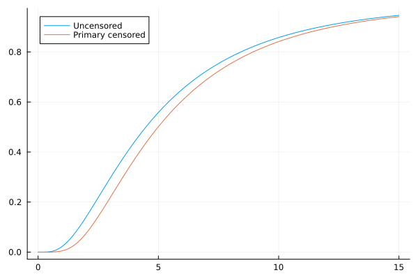
Truncation
Truncation is applied to ensure delays are within the specified range
If the maximum delay
We can apply truncation using the normal truncated function from Distributions.jl:
trunc_prim_dist = truncated(prim_dist, upper=10)Truncated(CensoredDistributions.PrimaryCensored{Distributions.LogNormal{Float64}, Distributions.Uniform{Float64}, CensoredDistributions.AnalyticalSolver{Integrals.QuadGKJL{typeof(LinearAlgebra.norm), Nothing}}}(
dist: Distributions.LogNormal{Float64}(μ=1.5, σ=0.75)
primary_event: Distributions.Uniform{Float64}(a=0.0, b=1.0)
method: CensoredDistributions.AnalyticalSolver{Integrals.QuadGKJL{typeof(LinearAlgebra.norm), Nothing}}(Integrals.QuadGKJL{typeof(LinearAlgebra.norm), Nothing}(7, LinearAlgebra.norm, nothing))
)
; upper=10.0)We can again sample from the distribution
Random.seed!(123)
rand(trunc_prim_dist, 10)
10-element Vector{Float64}:
3.3481078967458373
1.5170794868185762
6.8735941017127296
5.692020454408029
1.9657573450482368
7.8291474033596895
4.698045223247449
7.605147128720719
5.804377720321878
6.842209549861345or plot the CDFs of the different distributions:
x = 0:0.01:15
plot(x, cdf.(dist, x), label="Uncensored")
plot!(x, cdf.(prim_dist, x), label="Primary censored")
plot!(x, cdf.(trunc_prim_dist, x), label="Truncated and primary censored")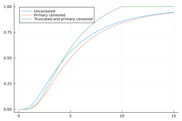
Secondary interval censoring
We can now apply secondary interval censoring using the interval_censored function. This censors observations to fall within specified intervals.
The secondary event censoring process rounds the truncated delays to the nearest secondary event window (
For discrete data or when working with specific time windows (such as daily reporting delays), this step is particularly important. The primary event censored probability mass function (PMF),
where
int_censored_dist = interval_censored(trunc_prim_dist, 1)CensoredDistributions.IntervalCensored{Distributions.Truncated{CensoredDistributions.PrimaryCensored{Distributions.LogNormal{Float64}, Distributions.Uniform{Float64}, CensoredDistributions.AnalyticalSolver{Integrals.QuadGKJL{typeof(LinearAlgebra.norm), Nothing}}}, Distributions.Continuous, Float64, Nothing, Float64}, Int64}(
dist: Truncated(CensoredDistributions.PrimaryCensored{Distributions.LogNormal{Float64}, Distributions.Uniform{Float64}, CensoredDistributions.AnalyticalSolver{Integrals.QuadGKJL{typeof(LinearAlgebra.norm), Nothing}}}(
dist: Distributions.LogNormal{Float64}(μ=1.5, σ=0.75)
primary_event: Distributions.Uniform{Float64}(a=0.0, b=1.0)
method: CensoredDistributions.AnalyticalSolver{Integrals.QuadGKJL{typeof(LinearAlgebra.norm), Nothing}}(Integrals.QuadGKJL{typeof(LinearAlgebra.norm), Nothing}(7, LinearAlgebra.norm, nothing))
)
; upper=10.0)
boundaries: 1
)Again we can sample from the distribution.
Random.seed!(123)
rand(int_censored_dist, 10)
10-element Vector{Float64}:
3.0
1.0
6.0
5.0
1.0
7.0
4.0
7.0
5.0
6.0or plot the CDFs of the different distributions.
x = 0:0.01:15
plot(x, cdf.(dist, x), label="Uncensored")
plot!(x, cdf.(prim_dist, x), label="Primary censored")
plot!(x, cdf.(trunc_prim_dist, x), label="Truncated and primary censored")
plot!(x, cdf.(int_censored_dist, x), label="Truncated, primary censored, and interval censored")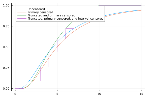
Neither the primary censored nor the interval censored distributions match the true distribution due to the censoring effects and truncation at the maximum observable delay, which biases both observed distributions towards shorter delays.
Convenience function: double_interval_censored
For common workflows involving the complete pipeline of primary censoring, truncation, and secondary interval censoring, the package provides a convenient double_interval_censored function that applies all transformations in the correct order (primary censoring → truncation → interval censoring):
# This is equivalent to the step-by-step approach above
double_censored_dist = double_interval_censored(Gamma(2, 1); upper=8, interval=2)
CensoredDistributions.IntervalCensored{Distributions.Truncated{CensoredDistributions.PrimaryCensored{Distributions.Gamma{Float64}, Distributions.Uniform{Float64}, CensoredDistributions.AnalyticalSolver{Integrals.QuadGKJL{typeof(LinearAlgebra.norm), Nothing}}}, Distributions.Continuous, Float64, Nothing, Float64}, Int64}(
dist: Truncated(CensoredDistributions.PrimaryCensored{Distributions.Gamma{Float64}, Distributions.Uniform{Float64}, CensoredDistributions.AnalyticalSolver{Integrals.QuadGKJL{typeof(LinearAlgebra.norm), Nothing}}}(
dist: Distributions.Gamma{Float64}(α=2.0, θ=1.0)
primary_event: Distributions.Uniform{Float64}(a=0.0, b=1.0)
method: CensoredDistributions.AnalyticalSolver{Integrals.QuadGKJL{typeof(LinearAlgebra.norm), Nothing}}(Integrals.QuadGKJL{typeof(LinearAlgebra.norm), Nothing}(7, LinearAlgebra.norm, nothing))
)
; upper=8.0)
boundaries: 2
)As with all the other functions, we can sample from the distribution
Random.seed!(123)
rand(double_censored_dist, 10)
10-element Vector{Float64}:
0.0
0.0
2.0
2.0
0.0
2.0
2.0
0.0
0.0
2.0or do any of the other common distribution operations.
Key package features
In addition to these main functions, the package also includes:
Distributions.jl integration: Full compatibility with the Distributions.jl ecosystem, supporting all standard distribution methods (
pdf,cdf,quantile,rand, etc.).Analytical solutions: For common combinations of primary event and delay distributions (e.g., uniform primary events with gamma, lognormal, or Weibull delays), analytical solutions provide significant computational speedups compared to numerical integration.
Automatic differentiation compatibility: Full support for automatic differentiation backends including ForwardDiff.jl, ReverseDiff.jl, Mooncake.jl, and Enzyme.jl for use in probabilistic programming and optimisation.
Type stability: Efficient implementation with type-stable operations for high-performance computation.
Learning more
Tutorials
For more information on the package and its integration with other packages, see the tutorials in this getting started section:
Analytical CDF solutions: Understanding analytical solutions for common distribution pairs
Fitting with Turing.jl: Bayesian inference with censored distributions
Exponentially tilted primary events: Understanding the impact of exponentially tilted primary events on primary event timing and the knock on impact to primary event censored distributions
Methodological background
For methodological background on delay distributions and censoring methods, see:
[1] - Provides detailed mathematical foundations and methodological guidance for delay distribution estimation.
[2] - Offers best practices and practical advice when estimating delay distributions from real-world data.
The primarycensored R package documentation provides additional theoretical context and examples.
References
S. W. Park, A. R. Akhmetzhanov, K. Charniga, A. Cori, J. Dushoff, S. Funk, K. M. Gostic, N. M. Linton, A. Lison, C. E. Overton, B. J. Cowling and S. Abbott. Estimating epidemiological delay distributions for infectious diseases, medRxiv preprint (2024).
K. Charniga, S. W. Park, A. R. Akhmetzhanov, A. Cori, J. Dushoff, S. Funk, K. M. Gostic, N. M. Linton, A. Lison, C. E. Overton, B. J. Cowling and S. Abbott. Best practices for estimating and reporting epidemiological delay distributions of infectious diseases. PLOS Computational Biology 20, e1012520 (2024).