Analytical CDF solutions for primary censored distributions

This tutorial demonstrates the analytical CDF solutions available in CensoredDistributions.jl. These analytical solutions provide significant performance improvements over numerical integration whilst maintaining machine precision accuracy.

Overview

Primary event censoring occurs when the exact time of an initiating event is unknown but falls within a known window. The observed time is the sum of:

1. The primary event time (uncertain, within a window)

2. A delay from the primary event to observation

CensoredDistributions.jl provides analytical solutions for certain distribution combinations, automatically using them when available for optimal performance.

Currently supported analytical solutions

Delay Distribution	Primary Distribution	Status
Gamma	Uniform	Analytical
LogNormal	Uniform	Analytical
Weibull	Uniform	Analytical
Others	Any	Numerical

These analytical solutions are based on the mathematical derivations implemented in the primarycensored R package, with detailed mathematical formulations available in their analytical solutions vignette.

Packages used

using CensoredDistributions
using Distributions
using BenchmarkTools
using CairoMakie
using AlgebraOfGraphics
using DataFramesMeta
using Printf
using Statistics
using Integrals

CairoMakie.activate!(type = "png", px_per_unit = 2)
set_theme!(theme_latexfonts(); fontsize = 14)

Automatic method selection

CensoredDistributions.jl automatically selects the appropriate method:

• Analytical solutions when available (optimal performance)

• Numerical integration as fallback

Let's see this in action with a Gamma distribution:

# Create a Gamma distribution for delays
gamma_delay = Gamma(2.0, 3.0)

# Primary event window (uniform over 1 day)
primary_uniform = Uniform(0.0, 1.0)

# Default: uses analytical solution for Gamma
pc_gamma_analytical = primary_censored(
    gamma_delay, primary_uniform
)

# Force numerical integration
pc_gamma_numerical = primary_censored(
    gamma_delay, primary_uniform; method = NumericSolver()
)

# Store solver types for display
solver_types = (
    analytical = typeof(pc_gamma_analytical.method),
    numerical = typeof(pc_gamma_numerical.method)
)

(analytical = AnalyticalSolver{CensoredDistributions.GaussLegendre{CensoredDistributions._GL{Vector{Float64}, Vector{Float64}}}}, numerical = NumericSolver{CensoredDistributions.GaussLegendre{CensoredDistributions._GL{Vector{Float64}, Vector{Float64}}}})

Let's verify both methods give the same results:

Show plotting code

x_compare = 0:0.5:10
cdf_analytical_vals = cdf.(pc_gamma_analytical, x_compare)
cdf_numerical_vals = cdf.(pc_gamma_numerical, x_compare)

cdf_compare_df = vcat(
    DataFrame(
        x = collect(x_compare),
        cdf = cdf_analytical_vals,
        method = "Analytical"
    ),
    DataFrame(
        x = collect(x_compare),
        cdf = cdf_numerical_vals,
        method = "Numerical"
    )
)

fig_cdf_compare = draw(
    data(cdf_compare_df) *
    mapping(:x, :cdf => "CDF", color = :method => "Method") *
    visual(Lines, linewidth = 2);
    axis = (title = "CDF Comparison: Analytical vs Numerical",)
);

fig_cdf_compare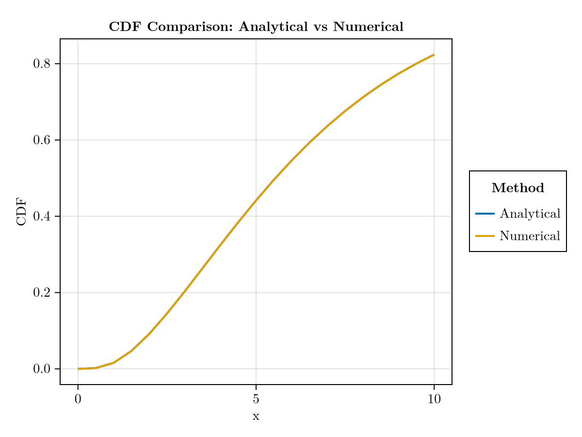

Performance comparison

Let's benchmark the performance difference between analytical and numerical methods:

# Create distributions for benchmarking
lognormal_delay = LogNormal(1.5, 0.75)
weibull_delay = Weibull(2.0, 1.5)

function benchmark_cdf_methods(
        dist, primary, name;
        x_values = [0.5, 1.0, 2.0, 5.0, 10.0, 20.0]
)
    # Create both versions
    d_analytical = primary_censored(dist, primary)
    d_numerical = primary_censored(
        dist, primary; method = NumericSolver()
    )

    # Benchmark at multiple x values
    speedups = Float64[]
    analytical_times = Float64[]
    numerical_times = Float64[]

    for x in x_values
        bench_analytical = @benchmark(cdf($d_analytical, $x), samples=100)
        bench_numerical = @benchmark(cdf($d_numerical, $x), samples=100)

        # Extract times in microseconds
        time_analytical = median(
            bench_analytical
        ).time / 1000
        time_numerical = median(
            bench_numerical
        ).time / 1000

        push!(analytical_times, time_analytical)
        push!(numerical_times, time_numerical)
        push!(
            speedups, time_numerical / time_analytical
        )
    end

    return (
        name = name,
        x_values = x_values,
        analytical_μs = analytical_times,
        numerical_μs = numerical_times,
        speedups = speedups,
        mean_speedup = mean(speedups),
        median_speedup = median(speedups),
        min_speedup = minimum(speedups),
        max_speedup = maximum(speedups)
    )
end

# Run benchmarks for all supported distributions
benchmark_results = [
    benchmark_cdf_methods(
        gamma_delay, primary_uniform, "Gamma"
    ),
    benchmark_cdf_methods(
        lognormal_delay, primary_uniform, "LogNormal"
    ),
    benchmark_cdf_methods(
        weibull_delay, primary_uniform, "Weibull"
    )
];

Show plotting code

# Summary statistics: build long-form DataFrames for AoG
dist_names = [r.name for r in benchmark_results]
mean_speedups = [r.mean_speedup for r in benchmark_results]
min_speedups = [r.min_speedup for r in benchmark_results]
max_speedups = [r.max_speedup for r in benchmark_results]

summary_df = DataFrame(
    distribution = dist_names,
    mean_speedup = mean_speedups,
    low = mean_speedups .- min_speedups,
    high = max_speedups .- mean_speedups
)

speedup_long_df = vcat(
    [DataFrame(
         distribution = r.name,
         x = r.x_values,
         speedup = r.speedups
     ) for r in benchmark_results]...
)

times_long_df = vcat(
    [vcat(
         DataFrame(
             distribution = r.name,
             x = r.x_values,
             time_us = r.analytical_μs,
             method = "Analytical"
         ),
         DataFrame(
             distribution = r.name,
             x = r.x_values,
             time_us = r.numerical_μs,
             method = "Numerical"
         )
     ) for r in benchmark_results]...
)

fig_benchmarks = Figure(size = (700, 900))

# Mean performance improvement (bar) with error bars
ax1 = Axis(
    fig_benchmarks[1, 1],
    title = "Mean Performance Improvement",
    ylabel = "Speedup Factor",
    xticks = (1:length(dist_names), dist_names)
)
barplot!(
    ax1, 1:length(dist_names), mean_speedups,
    color = :steelblue
)
errorbars!(
    ax1, 1:length(dist_names), mean_speedups,
    summary_df.low, summary_df.high;
    whiskerwidth = 10
)
for (i, speedup) in enumerate(mean_speedups)
    text!(
        ax1, i, speedup + 5;
        text = @sprintf("%.0fx", speedup),
        align = (:center, :bottom)
    )
end

# Speedup by x (log x)
draw!(
    fig_benchmarks[2, 1],
    data(speedup_long_df) *
    mapping(
        :x,
        :speedup => "Speedup Factor",
        color = :distribution => "Distribution"
    ) *
    (visual(Lines, linewidth = 2) +
     visual(Scatter, markersize = 8));
    axis = (
        title = "Speedup Factor by x Value",
        xscale = log10
    )
)

# Computation time comparison (log-log)
draw!(
    fig_benchmarks[3, 1],
    data(times_long_df) *
    mapping(
        :x,
        :time_us => "Time (microseconds)",
        color = :distribution => "Distribution",
        linestyle = :method => "Method"
    ) *
    visual(Lines, linewidth = 2);
    axis = (
        title = "Computation Time Comparison",
        xscale = log10,
        yscale = log10
    )
);

fig_benchmarks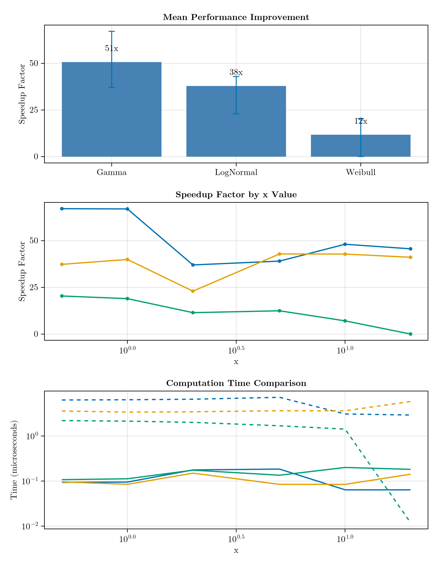

Accuracy verification

The analytical solutions maintain machine precision accuracy. Let's verify this:

function compare_accuracy(dist, primary, name, x_range)
    d_analytical = primary_censored(dist, primary)
    d_numerical = primary_censored(
        dist, primary; method = NumericSolver()
    )

    # Compute CDFs
    cdf_analytical = [cdf(d_analytical, x) for x in x_range]
    cdf_numerical = [cdf(d_numerical, x) for x in x_range]

    # Compute absolute errors
    abs_errors = abs.(cdf_analytical .- cdf_numerical)

    return (
        name = name,
        x = x_range,
        analytical = cdf_analytical,
        numerical = cdf_numerical,
        errors = abs_errors,
        max_error = maximum(abs_errors)
    )
end

x_test = range(0.1, 20, length = 100)

accuracy_gamma = compare_accuracy(
    gamma_delay, primary_uniform, "Gamma", x_test
)
accuracy_lognormal = compare_accuracy(
    lognormal_delay, primary_uniform,
    "LogNormal", x_test
)
accuracy_weibull = compare_accuracy(
    weibull_delay, primary_uniform,
    "Weibull", x_test
)

# Store accuracy results for display
max_errors = (
    gamma = accuracy_gamma.max_error,
    lognormal = accuracy_lognormal.max_error,
    weibull = accuracy_weibull.max_error
)

(gamma = 3.219646771412954e-15, lognormal = 2.886579864025407e-15, weibull = 1.1102230246251565e-15)

Show plotting code

# Build long-form DataFrames for CDF and error plots
cdf_accuracy_df = vcat(
    DataFrame(
        x = collect(accuracy_gamma.x),
        cdf = accuracy_gamma.analytical,
        distribution = "Gamma"
    ),
    DataFrame(
        x = collect(accuracy_lognormal.x),
        cdf = accuracy_lognormal.analytical,
        distribution = "LogNormal"
    ),
    DataFrame(
        x = collect(accuracy_weibull.x),
        cdf = accuracy_weibull.analytical,
        distribution = "Weibull"
    )
)

error_df = vcat(
    DataFrame(
        x = collect(accuracy_gamma.x),
        err = accuracy_gamma.errors .+ 1e-17,
        distribution = "Gamma"
    ),
    DataFrame(
        x = collect(accuracy_lognormal.x),
        err = accuracy_lognormal.errors .+ 1e-17,
        distribution = "LogNormal"
    ),
    DataFrame(
        x = collect(accuracy_weibull.x),
        err = accuracy_weibull.errors .+ 1e-17,
        distribution = "Weibull"
    )
)

fig_acc = Figure(size = (700, 600))

draw!(
    fig_acc[1, 1],
    data(cdf_accuracy_df) *
    mapping(
        :x,
        :cdf => "CDF",
        color = :distribution => "Distribution"
    ) *
    visual(Lines, linewidth = 2);
    axis = (
        title = "CDF Comparison: Analytical vs Numerical",
    )
)

draw!(
    fig_acc[2, 1],
    data(error_df) *
    mapping(
        :x,
        :err => "Absolute Error",
        color = :distribution => "Distribution"
    ) *
    visual(Lines, linewidth = 2);
    axis = (
        title = "Absolute Error: |Analytical - Numerical|",
        yscale = log10,
        limits = (nothing, (1e-17, 1e-13))
    )
);

fig_acc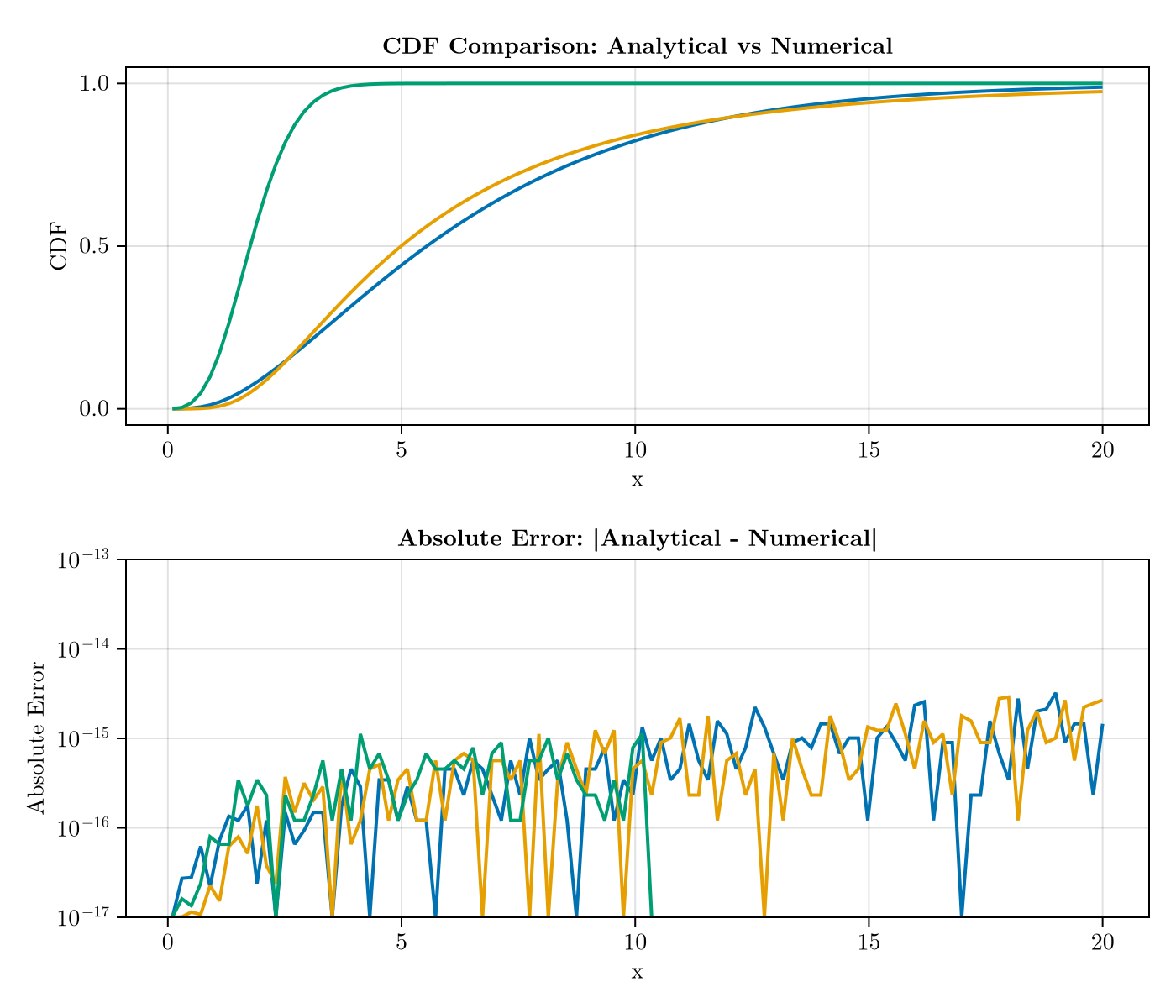

Exploring available methods

You can use Julia's methods function to discover which distribution combinations have analytical solutions:

# Find all analytical CDF implementations
analytical_methods = methods(
    CensoredDistributions.primarycensored_cdf,
    (
        Any, Any, Real,
        CensoredDistributions.AnalyticalSolver
    )
)

# 4 methods for generic function primarycensored_cdf from CensoredDistributions:

• primarycensored_cdf(dist::Distributions.Gamma, primary_event::Distributions.Uniform, x::Real, ::AnalyticalSolver) in CensoredDistributions at /home/runner/work/CensoredDistributions.jl/CensoredDistributions.jl/src/censoring/primarycensored_cdf.jl:323
• primarycensored_cdf(dist::Distributions.LogNormal, primary_event::Distributions.Uniform, x::Real, ::AnalyticalSolver) in CensoredDistributions at /home/runner/work/CensoredDistributions.jl/CensoredDistributions.jl/src/censoring/primarycensored_cdf.jl:373
• primarycensored_cdf(dist::Distributions.Weibull, primary_event::Distributions.Uniform, x::Real, ::AnalyticalSolver) in CensoredDistributions at /home/runner/work/CensoredDistributions.jl/CensoredDistributions.jl/src/censoring/primarycensored_cdf.jl:415
• primarycensored_cdf(dist::D1, primary_event::D2, x::Real, method::AnalyticalSolver) where {D1<:(Distributions.UnivariateDistribution), D2<:(Distributions.UnivariateDistribution)} in CensoredDistributions at /home/runner/work/CensoredDistributions.jl/CensoredDistributions.jl/src/censoring/primarycensored_cdf.jl:162

The above shows all methods defined for primarycensored_cdf with an AnalyticalSolver. Each method signature shows which distribution combinations have analytical solutions implemented.

Custom solver options

You can also customise the numerical solver when needed:

# Create an exponential distribution
# (no analytical solution available)
exponential_delay = Exponential(2.0)

# Default solver (GaussLegendre, AD-friendly)
pc_default = primary_censored(
    exponential_delay, primary_uniform
)

# Custom solver (HCubatureJL for multidimensional)
pc_custom = primary_censored(
    exponential_delay, primary_uniform;
    solver = HCubatureJL()
)

# With analytical solutions available, you can specify
# a custom solver (used if you force numeric or for
# distributions without analytical solutions)
pc_gamma_custom = primary_censored(
    gamma_delay, primary_uniform;
    solver = HCubatureJL()
)

# Store solver information for display
solver_info = (
    default = typeof(pc_default.method.solver),
    custom = typeof(pc_custom.method.solver)
)

(default = CensoredDistributions.GaussLegendre{CensoredDistributions._GL{Vector{Float64}, Vector{Float64}}}, custom = Integrals.HCubatureJL{typeof(LinearAlgebra.norm), Nothing})

Implementing new analytical solutions

If you have derived an analytical solution for a new distribution combination, you can extend the package by defining a new method for primarycensored_cdf. The key steps are:

1. Derive the mathematical formula following the methodology in the primarycensored R package vignette

2. Define a new method for the specific distribution types making sure to define it for the AnalyticalSolver method.

3. Use log-space computations with LogExpFunctions.jl for numerical stability

4. Test thoroughly against numerical integration

For detailed implementation guidance, see the existing implementations in the source code at src/censoring/primarycensored_cdf.jl.

Summary

The analytical CDF solutions in CensoredDistributions.jl provide:

1. Automatic optimisation: The package automatically uses analytical solutions when available

2. Significant speedup: 15-100x performance improvement over numerical integration

3. Machine precision accuracy: Errors typically < 1e-15

4. Consistent API: Same interface whether using analytical or numerical methods

5. Flexibility: Can force numerical methods or use custom solvers when needed

References

• primarycensored R package: Reference implementation with mathematical derivations

• Analytical solutions vignette: Detailed mathematical formulations

• [1]: Background on truncation and double interval censoring