How exponentially tilted primary events affect observed delay distributions
Introduction
What are we going to do in this exercise
We'll demonstrate how epidemic growth creates additional bias in observed delay distributions through primary event censoring - distinct from truncation bias. We'll cover:
Exponentially tilted vs Uniform primary events
Double interval censoring effects
Impact on delay distributions
What might I need to know before starting
This tutorial builds on Getting Started with CensoredDistributions.jl and focusses on exponentially tilted primary events - when primary events occur non-uniformly within observation windows (due here to exponential dynamics).
During epidemic growth/decline, primary events don't occur uniformly within our observation window:
Growth phase: Recent primary events over-represented leading to shorter observed delays
Decline phase: Older primary events more represented leading to longer observed delays
Steady state: Uniform timing leading to minimal additional bias
Setup
Packages used
using CensoredDistributions
using Distributions
using CairoMakie
using AlgebraOfGraphics
using DataFramesMeta
using KernelDensity
using Statistics
using Random

CairoMakie.activate!(type = "png", px_per_unit = 2)
set_theme!(theme_latexfonts(); fontsize = 14)

Random.seed!(123)Random.TaskLocalRNG()Simulated scenarios
We'll examine epidemic phase bias using a realistic scenario:
True incubation period: Gamma(4.0, 1.5) with mean 6.0 days
Primary event windows: 7-day observation periods
Growth rate scenarios: r in
true_delay = Gamma(4.0, 1.5);Part 1: Exponentially tilted vs uniform primary events
First, we compare how exponentially tilted distributions with different growth rates shape primary event timing compared to uniform (steady state) patterns.
window_length = 7
scenarios_df = @chain DataFrame(
    name = [
        "Decline 10%", "Decline 5%",
        "Steady", "Growth 5%", "Growth 10%"
    ],
    r = [-0.10, -0.05, 0.0, 0.05, 0.10],
    color = [:darkgreen, :lightgreen, :blue, :orange, :red]
) begin
    @transform :window = window_length
end

@chain scenarios_df begin
    @transform! :primary_event = ExponentiallyTilted.(0.0, :window, :r)
    @transform! :uniform_ref = Uniform.(0.0, :window)
end| Row | name | r | color | window | primary_event | uniform_ref |
|---|---|---|---|---|---|---|
| String | Float64 | Symbol | Int64 | Exponent… | Uniform… | |
| 1 | Decline 10% | -0.1 | darkgreen | 7 | ExponentiallyTilted{Float64}(min=0.0, max=7.0, r=-0.1) | Distributions.Uniform{Float64}(a=0.0, b=7.0) |
| 2 | Decline 5% | -0.05 | lightgreen | 7 | ExponentiallyTilted{Float64}(min=0.0, max=7.0, r=-0.05) | Distributions.Uniform{Float64}(a=0.0, b=7.0) |
| 3 | Steady | 0.0 | blue | 7 | ExponentiallyTilted{Float64}(min=0.0, max=7.0, r=0.0) | Distributions.Uniform{Float64}(a=0.0, b=7.0) |
| 4 | Growth 5% | 0.05 | orange | 7 | ExponentiallyTilted{Float64}(min=0.0, max=7.0, r=0.05) | Distributions.Uniform{Float64}(a=0.0, b=7.0) |
| 5 | Growth 10% | 0.1 | red | 7 | ExponentiallyTilted{Float64}(min=0.0, max=7.0, r=0.1) | Distributions.Uniform{Float64}(a=0.0, b=7.0) |
Created 5 epidemic scenarios for comparison. Now lets plot the primary event timing distributions.
Show plotting code
x_primary = range(0, window_length, length = 100)

primary_pdf_df = vcat(
    [DataFrame(
         x = x_primary,
         pdf = pdf.(row.primary_event, x_primary),
         scenario = "$(row.name) (r=$(row.r))"
     ) for row in eachrow(scenarios_df)]...,
    DataFrame(
        x = x_primary,
        pdf = pdf.(Uniform(0.0, window_length), x_primary),
        scenario = "Uniform (reference)"
    )
)

fig_primary_events = draw(
    data(primary_pdf_df) *
    mapping(
        :x => "Days before observation end",
        :pdf => "Probability density",
        color = :scenario => "Scenario"
    ) *
    visual(Lines, linewidth = 3);
    figure = (size = (700, 400),),
    axis = (title = "Primary Event Timing: " *
                    "ExponentiallyTilted vs Uniform",)
);fig_primary_events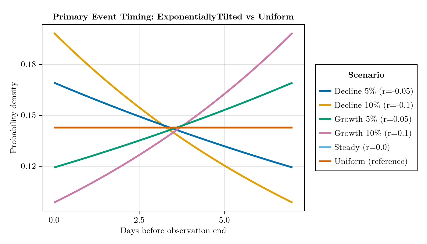
Part 2: Double interval censoring - primary + secondary windows
Now we demonstrate the double interval censoring concept: primary events occur within surveillance-defined primary windows, but during epidemics their timing distribution becomes non-uniform (ExponentiallyTilted), then we observe delays within secondary windows (surveillance window minus primary event time). For the secondary event the distribution doesn't impact what we observe (see references for why).
n_samples = 50_000
secondary_window = 7.0

censoring_windows_df = @chain scenarios_df begin
    vcat([DataFrame(
              name = fill(row.name, n_samples),
              r = fill(row.r, n_samples),
              primary_time = rand(
                  row.primary_event, n_samples
              )
          ) for row in eachrow(_)]...)
    @transform :effective_window = secondary_window .- :primary_time
end;
Now we can plot the distribution of effective censoring windows by scenario.
Show plotting code
# AoG's density() analysis returns a 2D grid that visual(Lines)
# can't render, so compute the KDE per scenario up-front and feed
# the resulting (x, density) curves into a standard AoG pipeline.
effective_windows_kde_df = vcat([begin
                                     sub = filter(
                                         :name => ==(scen),
                                         censoring_windows_df
                                     )
                                     k = kde(sub.effective_window)
                                     DataFrame(
                                         x = collect(k.x),
                                         density = k.density,
                                         name = scen
                                     )
                                 end
                                 for scen in scenarios_df.name]...)

fig_effective_windows = draw(
    data(effective_windows_kde_df) *
    mapping(
        :x => "Effective censoring window (days)",
        :density => "Density",
        color = :name => "Scenario"
    ) *
    visual(Lines, linewidth = 2);
    figure = (size = (700, 400),),
    axis = (title = "Distribution of Effective " *
                    "Censoring Windows by Epidemic Phase",)
);fig_effective_windows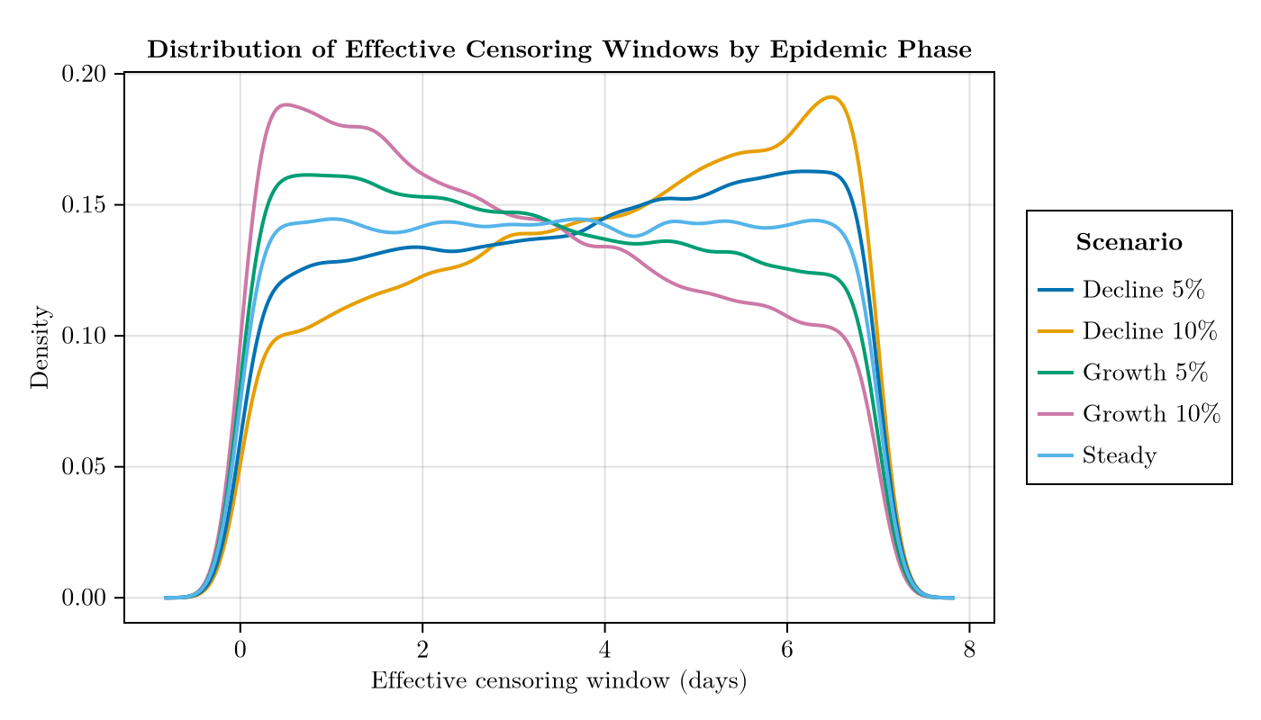
Part 3: Impact on censored delay distributions
Now we examine how epidemic phase bias affects the delays we might observe. We start with the primary censored delay distributions. Note that most of the time, we won't observe these continuous distributions as the secondary event will also be censored.
@chain scenarios_df begin
    @transform! :censored_dist = primary_censored.(
        Ref(true_delay), :primary_event
    )
end;
Show plotting code
x_delay = range(0, 15, length = 100)

delay_pdf_df = vcat(
    DataFrame(
        x = x_delay,
        pdf = pdf.(true_delay, x_delay),
        scenario = "True distribution"
    ),
    [DataFrame(
         x = x_delay,
         pdf = pdf.(row.censored_dist, x_delay),
         scenario = "$(row.name) (r=$(row.r))"
     ) for row in eachrow(scenarios_df)]...
)

fig_delay_pdfs = draw(
    data(delay_pdf_df) *
    mapping(
        :x => "Delay (days)",
        :pdf => "Probability density",
        color = :scenario => "Scenario"
    ) *
    visual(Lines, linewidth = 2);
    figure = (size = (700, 400),),
    axis = (title = "Observed vs True Delay Distributions",)
);fig_delay_pdfs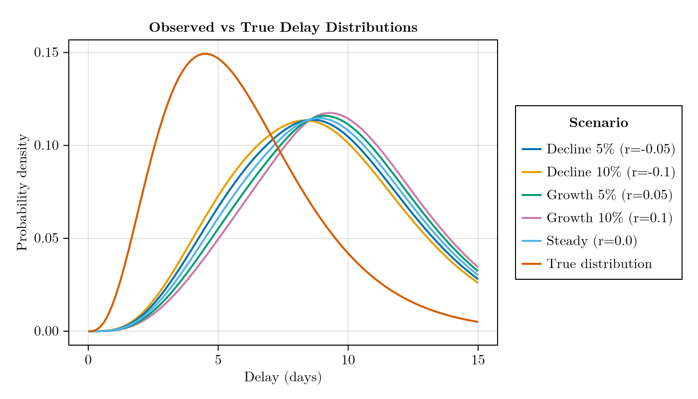
We can also plot the impact on the double censored distribution (which is what we would often observe). Here we show the CDF.
@chain scenarios_df begin
    @rtransform! :double_censored_dist = double_interval_censored(
        true_delay;
        primary_event = :primary_event,
        interval = secondary_window
    )
end;
Show plotting code
x_delay_d = range(0, 40, length = 100)

double_cdf_df = vcat(
    DataFrame(
        x = x_delay_d,
        cdf = cdf.(true_delay, x_delay_d),
        scenario = "True distribution"
    ),
    [DataFrame(
         x = x_delay_d,
         cdf = cdf.(
             row.double_censored_dist, x_delay_d
         ),
         scenario = "$(row.name) Double (r=$(row.r))"
     ) for row in eachrow(scenarios_df)]...
)

fig_double_cdfs = draw(
    data(double_cdf_df) *
    mapping(
        :x => "Delay (days)",
        :cdf => "Cumulative probability",
        color = :scenario => "Scenario"
    ) *
    visual(Lines, linewidth = 2);
    figure = (size = (700, 400),),
    axis = (title = "Double vs Single Interval " *
                    "Censored Distributions",)
);fig_double_cdfs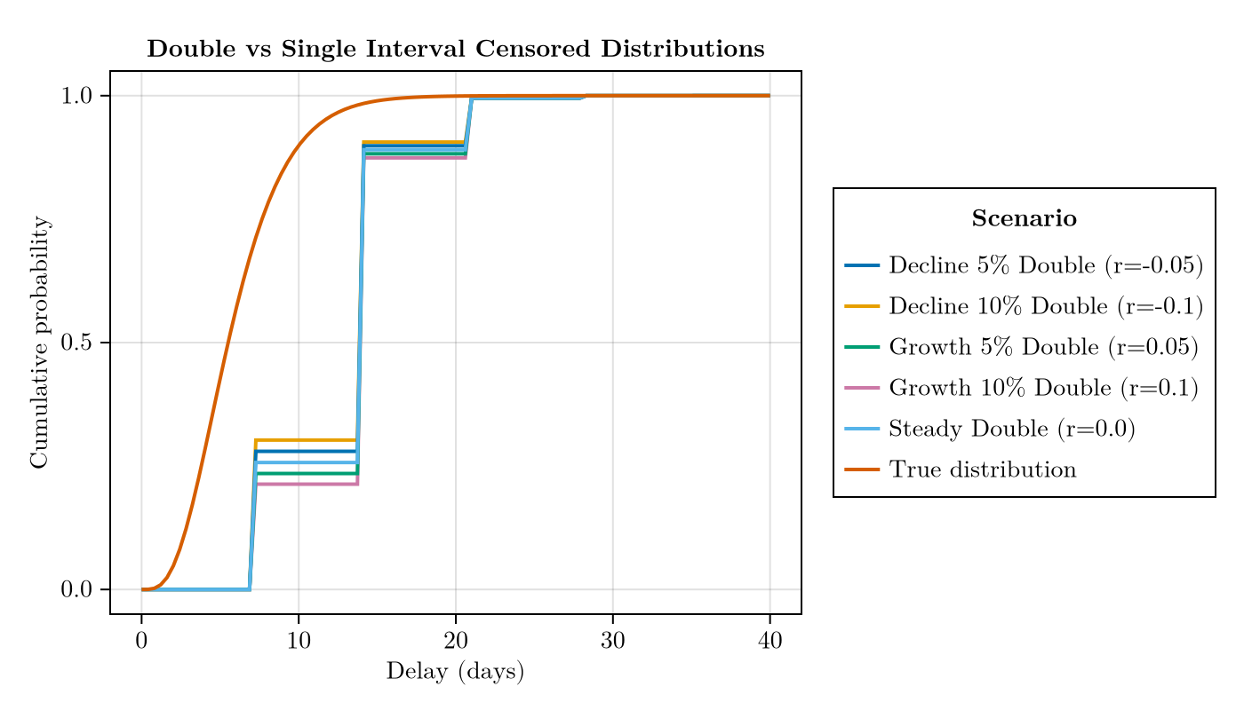
Key insights
- Primary event bias is distinct from truncation bias:
Occurs regardless of the primary event distribution but is more complex when the primary event distribution is non-uniform.
Growth phase: Recent primary events over-represented leading to shorter observed delays
Decline phase: Older primary events more represented leading to longer observed delays
- Two key factors control bias magnitude:
Growth rate magnitude: Stronger growth (larger |r|) creates more divergence from the uniform case
Window length: Longer windows increases divergence for same growth rate
- When to use
ExponentiallyTilted:
Most important when primary censoring intervals are wide (multi-day windows)
For daily primary censoring and moderate epidemic growth, Uniform distributions are often a reasonable approximation
Key benefit of Uniform: Analytical solutions available that are much faster computationally
Use
ExponentiallyTiltedwhen precision is critical, the computational cost is acceptable, and the growth rate is relatively well known.
References
[1]: "Estimating epidemiological delay distributions for infectious diseases"
[2]: "Best practices for estimating and reporting epidemiological delay distributions"
SISMID Tutorial: Interactive bias demonstrations