Fitting CensoredDistributions.jl modified distributions with Turing.jl

Introduction

What are we going to do in this exercise

We'll demonstrate how to use CensoredDistributions.jl in conjunction with Turing.jl for Bayesian inference of epidemiological delay distributions. We'll cover the following key points:

Defining a simple delay distribution model without observation processes.
Exploring the prior distribution of this model.
Defining a Bayesian model that incorporates double censoring and right truncation
Generating synthetic data from the model using fixed parameters
Fitting a naive model that ignores censoring
Fitting a model that accounts for secondary event censoring and truncation but not primary event censoring.
Fitting the full model that accounts for double censoring and right truncation.

What might I need to know before starting

This tutorial builds on the concepts introduced in Getting Started with CensoredDistributions.jl.

Packages used

We use CairoMakie for plotting, Turing for probabilistic programming, Chain.jl for data pipeline workflows, DataFramesMeta, Random, and StatsBase.

begin
    using DataFramesMeta
    using Turing
    using DynamicPPL
    using Distributions
    using Random
    using CairoMakie, PairPlots
    using StatsBase
    using CensoredDistributions
end

Generate synthetic data using Turing model simulation

We'll generate synthetic data by simulating from our Turing model with known true parameters. This approach ensures consistency between the data generation process and the model we'll use for inference, demonstrating how Turing models can be used for both simulation and fitting.

The proper Turing simulation approach:

Define a Turing model that incorporates double censoring and right truncation
Create a model instance with missing observations for simulation
Use DynamicPPL's fix function to set parameters to their true values
Sample from the prior predictive distribution by calling the model as a function

Random.seed!(123) # Set seed for reproducibility

TaskLocalRNG()

Define the true parameters for generating synthetic data

We start by defining the number of samples and the true parameters of the lognormal.

n = 2000;

meanlog = 1.5;

sdlog = 0.75;

Now we can define a lognormal distribution using Distributions.jl.

true_dist = LogNormal(meanlog, sdlog);

For each individual we now sample a primary and secondary event window as well as a relative observation time (relative to their censored primary event).

Define a reusable submodel for the latent delay distribution

To avoid code duplication across our models, we define a submodel that encapsulates the latent delay distribution parameters. This pattern allows us to reuse the same prior structure across all our models:

@model function latent_delay_dist()
    mu ~ Normal(1.0, 2.0);
    sigma ~ truncated(Normal(0.5, 1); lower = 0.0)
    return LogNormal(mu, sigma)
end

latent_delay_dist (generic function with 2 methods)

and define a helper function to standardize our pairplot visualizations across all model fits:

function plot_fit_with_truth(chain, truth_dict)
    f = pairplot(
        chain,
        PairPlots.Truth(
            truth_dict,
            label = "True Values"
        )
    )
    return f
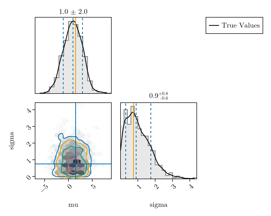
end

plot_fit_with_truth (generic function with 1 method)

Prior predictive checks using pairplot

First, let's visualise the prior predictive distribution by sampling from the instantiated model with uninformative priors and comparing against our true parameters. This shows what the model believes before seeing any data.

begin
    # Sample from the latent delay distribution prior
    latent_prior_samples = sample(latent_delay_dist(), Prior(), 1000)

    # Visualize the prior distribution
    plot_fit_with_truth(latent_prior_samples, (; mu = meanlog, sigma = sdlog))
end

Define the double censored model for simulation and fitting

Now we define our full model that incorporates double censoring and right truncation. This model uses the latent_delay_dist() submodel via to_submodel() to include the delay distribution parameters. It also uses our double_interval_censored() function to define each double censored and right truncated delay:

@model function CensoredDistributions_model(y, n, primary_dists, sws, Ds)
    dist ~ to_submodel(latent_delay_dist())

    pcens_dists = map(primary_dists, Ds, sws) do pe, D, sw
        double_interval_censored(
            dist; primary_event = pe, upper = D, interval = sw)
    end

    y ~ weight(pcens_dists, n)
    return y
end

CensoredDistributions_model (generic function with 2 methods)

We also need to define our simulated observation windows for each observed delay and the amount of censored time in which events have been observed (required to adjust for truncation). We do this in a data frame.

simulated_scenario = DataFrame(
    pwindow = rand(1:2, n),
    swindow = rand(1:2, n),
    obs_time = rand(8:12, n)
)

	pwindow	swindow	obs_time
1	2	1	11
2	1	1	10
3	2	1	8
4	1	1	8
5	2	2	10
6	2	2	11
7	2	1	8
8	1	1	11
9	1	2	10
10	2	2	10
...
2000	1	1	11

Simulate from the double censored distribution for each individual

Using the double censored model, we simulate data by sampling from the model using known true parameters. We use Turing's proper simulation approach with DynamicPPL's fix function to set parameters to their true values and sample from the prior predictive distribution. We first define a set of primary event distributions:

# Create primary event distributions from pwindows
@chain simulated_scenario begin
    @transform! :primary_dist = Uniform.(0.0, :pwindow)
end;

Then we can define the model using our observation windows.

model_for_simulation = @with simulated_scenario begin
    CensoredDistributions_model(
        missing, ones(n), :primary_dist, :swindow, :obs_time)
end

Model{typeof(CensoredDistributions_model), (:y, :n, :primary_dists, :sws, :Ds), (), (:y,), Tuple{Missing, Vector{Float64}, Vector{Uniform{Float64}}, Vector{Int64}, Vector{Int64}}, Tuple{}, DefaultContext}(CensoredDistributions_model, (y = missing, n = [1.0, 1.0, 1.0, 1.0, 1.0, 1.0, 1.0, 1.0, 1.0, 1.0  …  1.0, 1.0, 1.0, 1.0, 1.0, 1.0, 1.0, 1.0, 1.0, 1.0], primary_dists = Uniform{Float64}[Distributions.Uniform{Float64}(a=0.0, b=2.0), Distributions.Uniform{Float64}(a=0.0, b=1.0), Distributions.Uniform{Float64}(a=0.0, b=2.0), Distributions.Uniform{Float64}(a=0.0, b=1.0), Distributions.Uniform{Float64}(a=0.0, b=2.0), Distributions.Uniform{Float64}(a=0.0, b=2.0), Distributions.Uniform{Float64}(a=0.0, b=2.0), Distributions.Uniform{Float64}(a=0.0, b=1.0), Distributions.Uniform{Float64}(a=0.0, b=1.0), Distributions.Uniform{Float64}(a=0.0, b=2.0)  …  Distributions.Uniform{Float64}(a=0.0, b=2.0), Distributions.Uniform{Float64}(a=0.0, b=1.0), Distributions.Uniform{Float64}(a=0.0, b=2.0), Distributions.Uniform{Float64}(a=0.0, b=1.0), Distributions.Uniform{Float64}(a=0.0, b=2.0), Distributions.Uniform{Float64}(a=0.0, b=2.0), Distributions.Uniform{Float64}(a=0.0, b=2.0), Distributions.Uniform{Float64}(a=0.0, b=2.0), Distributions.Uniform{Float64}(a=0.0, b=1.0), Distributions.Uniform{Float64}(a=0.0, b=1.0)], sws = [1, 1, 1, 1, 2, 2, 1, 1, 2, 2  …  2, 1, 2, 1, 2, 2, 1, 1, 1, 1], Ds = [11, 10, 8, 8, 10, 11, 8, 11, 10, 10  …  9, 9, 12, 11, 11, 10, 9, 12, 8, 11]), NamedTuple(), DefaultContext())

We can then fix our priors based on the known values.


fixed_model = fix(
    model_for_simulation,
    (@varname(dist.mu) => meanlog, @varname(dist.sigma) => sdlog))

Model{typeof(CensoredDistributions_model), (:y, :n, :primary_dists, :sws, :Ds), (), (:y,), Tuple{Missing, Vector{Float64}, Vector{Uniform{Float64}}, Vector{Int64}, Vector{Int64}}, Tuple{}, DynamicPPL.FixedContext{Dict{VarName{:dist}, Float64}, DefaultContext}}(CensoredDistributions_model, (y = missing, n = [1.0, 1.0, 1.0, 1.0, 1.0, 1.0, 1.0, 1.0, 1.0, 1.0  …  1.0, 1.0, 1.0, 1.0, 1.0, 1.0, 1.0, 1.0, 1.0, 1.0], primary_dists = Uniform{Float64}[Distributions.Uniform{Float64}(a=0.0, b=2.0), Distributions.Uniform{Float64}(a=0.0, b=1.0), Distributions.Uniform{Float64}(a=0.0, b=2.0), Distributions.Uniform{Float64}(a=0.0, b=1.0), Distributions.Uniform{Float64}(a=0.0, b=2.0), Distributions.Uniform{Float64}(a=0.0, b=2.0), Distributions.Uniform{Float64}(a=0.0, b=2.0), Distributions.Uniform{Float64}(a=0.0, b=1.0), Distributions.Uniform{Float64}(a=0.0, b=1.0), Distributions.Uniform{Float64}(a=0.0, b=2.0)  …  Distributions.Uniform{Float64}(a=0.0, b=2.0), Distributions.Uniform{Float64}(a=0.0, b=1.0), Distributions.Uniform{Float64}(a=0.0, b=2.0), Distributions.Uniform{Float64}(a=0.0, b=1.0), Distributions.Uniform{Float64}(a=0.0, b=2.0), Distributions.Uniform{Float64}(a=0.0, b=2.0), Distributions.Uniform{Float64}(a=0.0, b=2.0), Distributions.Uniform{Float64}(a=0.0, b=2.0), Distributions.Uniform{Float64}(a=0.0, b=1.0), Distributions.Uniform{Float64}(a=0.0, b=1.0)], sws = [1, 1, 1, 1, 2, 2, 1, 1, 2, 2  …  2, 1, 2, 1, 2, 2, 1, 1, 1, 1], Ds = [11, 10, 8, 8, 10, 11, 8, 11, 10, 10  …  9, 9, 12, 11, 11, 10, 9, 12, 8, 11]), NamedTuple(), FixedContext(Dict{AbstractPPL.VarName{:dist}, Float64}(dist.sigma => 0.75, dist.mu => 1.5), DynamicPPL.DefaultContext()))

DynamicPPL.fixed(fixed_model)

Dict{VarName{:dist}, Float64} with 2 entries:
  dist.sigma => 0.75
  dist.mu    => 1.5

To simulate from this model all we need to do is call it:

observed_delays = fixed_model()

2000-element Vector{Float64}:
 8.0
 3.0
 5.0
 3.0
 8.0
 0.0
 3.0
 ⋮
 4.0
 4.0
 3.0
 2.0
 4.0
 1.0

Now lets create a simulated data frame using our scenarios data frame and simulated data.

simulated_data = @chain simulated_scenario begin
    @transform :observed_delay = observed_delays
    @transform :observed_delay_upper = :observed_delay .+ :swindow
end;

Visualise the simulated data

To make handling the data easier and later to speed up our models we first create a dataframe with the data we just generated, aggregated to unique combinations and count occurrences.

simulated_counts = @chain simulated_data begin
    @groupby All()
    @combine :n = length(:pwindow)
end

	pwindow	swindow	obs_time	primary_dist	observed_delay	observed_delay_upper	n
1	2	1	11	Distributions.Uniform{Float64}(a=0.0, b=2.0)	8.0	9.0	8
2	1	1	10	Distributions.Uniform{Float64}(a=0.0, b=1.0)	3.0	4.0	24
3	2	1	8	Distributions.Uniform{Float64}(a=0.0, b=2.0)	5.0	6.0	15
4	1	1	8	Distributions.Uniform{Float64}(a=0.0, b=1.0)	3.0	4.0	13
5	2	2	10	Distributions.Uniform{Float64}(a=0.0, b=2.0)	8.0	10.0	17
6	2	2	11	Distributions.Uniform{Float64}(a=0.0, b=2.0)	0.0	2.0	4
7	2	1	8	Distributions.Uniform{Float64}(a=0.0, b=2.0)	3.0	4.0	25
8	1	1	11	Distributions.Uniform{Float64}(a=0.0, b=1.0)	7.0	8.0	8
9	1	2	10	Distributions.Uniform{Float64}(a=0.0, b=1.0)	4.0	6.0	35
10	1	1	9	Distributions.Uniform{Float64}(a=0.0, b=1.0)	4.0	5.0	15
...
144	2	1	10	Distributions.Uniform{Float64}(a=0.0, b=2.0)	0.0	1.0	1

Now let's compare the samples with and without double interval censoring to the true distribution. First let's calculate the empirical CDF:

empirical_cdf_obs = @with(simulated_counts, ecdf(:observed_delay, weights = :n));

# Create a sequence of x values for the theoretical CDF
x_seq = @with simulated_counts begin
    range(minimum(:observed_delay), stop = maximum(:observed_delay) + 2, length = 100);
end

0.0:0.13131313131313133:13.0

begin
    # Calculate theoretical CDF using true log-normal distribution
    theoretical_cdf = @chain x_seq begin
        cdf.(true_dist, _)
    end;

    # Generate uncensored samples from the true distribution for comparison
    uncensored_samples = rand(true_dist, n);
    empirical_cdf_uncensored = ecdf(uncensored_samples);
end

ECDF{Vector{Float64}, Weights{Float64, Float64, Vector{Float64}}}([0.4070845594522205, 0.4092547609739798, 0.5410877914971672, 0.6147424004583137, 0.6168667235012328, 0.6503939798846371, 0.6673341355239283, 0.7261027423293577, 0.7261365044880947, 0.7335554368605154  …  27.194546062759702, 27.21281836005962, 28.976245628839653, 33.55236096071977, 34.34031231478969, 34.98956743654614, 36.173400053297016, 40.243111248984356, 40.25349036376026, 43.72612482134988], Float64[])

let
    f = Figure()
    ax = Axis(f[1, 1],
        title = "Comparison of Censored vs Uncensored vs Theoretical CDF",
        ylabel = "Cumulative Probability",
        xlabel = "Delay"
    )
    scatter!(
        ax,
        x_seq,
        empirical_cdf_obs.(x_seq),
        label = "Empirical CDF (Censored)",
        color = :blue
    )
    scatter!(
        ax,
        x_seq,
        empirical_cdf_uncensored.(x_seq),
        label = "Empirical CDF (Uncensored)",
        color = :red,
        marker = :cross
    )
    lines!(ax, x_seq, theoretical_cdf, label = "Theoretical CDF",
        color = :black, linewidth = 2)
    vlines!(ax, [mean(simulated_data.observed_delay)], color = :blue, linestyle = :dash,
        label = "Censored mean", linewidth = 2)
    vlines!(ax, [mean(uncensored_samples)], color = :red, linestyle = :dash,
        label = "Uncensored mean", linewidth = 2)
    vlines!(ax, [mean(true_dist)], linestyle = :dash,
        label = "Theoretical mean", color = :black, linewidth = 2)
    axislegend(position = :rb)

    f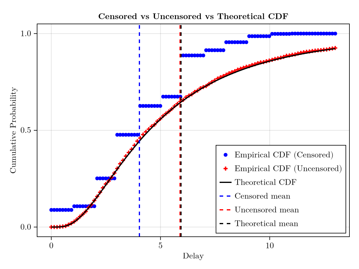
end

Fitting a naive model using Turing

We'll now fit a naive model that ignores the censoring process. This model treats the observed delay data as if it came directly from the uncensored delay distribution, providing a baseline for comparison.

@model function naive_model(y, n)
    dist ~ to_submodel(latent_delay_dist())
    y ~ weight(dist, n)
end

naive_model (generic function with 2 methods)

Now lets instantiate this model with data. Note we add a small constant to avoid issues at zero for this simple model.

naive_mdl = @with(simulated_counts, naive_model(:observed_delay .+ 1e-6, :n))

Model{typeof(naive_model), (:y, :n), (), (), Tuple{Vector{Float64}, Vector{Int64}}, Tuple{}, DefaultContext}(naive_model, (y = [8.000001, 3.000001, 5.000001, 3.000001, 8.000001, 1.0e-6, 3.000001, 7.000001, 4.000001, 4.000001  …  1.0e-6, 1.0e-6, 1.000001, 9.000001, 11.000001, 11.000001, 9.000001, 1.0e-6, 10.000001, 1.0e-6], n = [8, 24, 15, 13, 17, 4, 25, 8, 35, 15  …  1, 5, 2, 2, 1, 2, 2, 3, 3, 1]), NamedTuple(), DefaultContext())

and now let's fit the compiled model.

naive_fit = sample(naive_mdl, NUTS(), MCMCThreads(), 500, 4);

summarize(naive_fit)

	parameters	mean	std	mcse	ess_bulk	ess_tail	rhat	ess_per_sec
1	Symbol("dist.mu")	0.829945	0.058211	0.0014157	1692.72	1438.19	1.00348	271.793
2	Symbol("dist.sigma")	2.71551	0.043169	0.00112538	1462.79	1164.63	1.00146	234.873

plot_fit_with_truth(naive_fit, Dict("dist.mu" => meanlog, "dist.sigma" => sdlog))

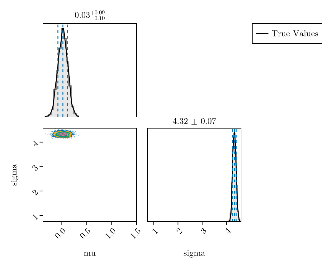
We see that the model has converged and the diagnostics look good. However, just from the model posterior summary we see that we might not be very happy with the fit. mu is smaller than the target 1.5 and sigma is larger than the target 0.75.

Fitting a truncation-adjusted interval model

Now let's fit an intermediate model that accounts for interval censoring and right truncation but ignores the primary censoring process. This provides a comparison point between the naive model and the full model.

@model function interval_only_model(y, n, sws, Ds)
    dist ~ to_submodel(latent_delay_dist())
    icens_dists = map(Ds, sws) do D, sw
        truncated(interval_censored(dist, sw), upper = D)
    end
    y ~ weight(icens_dists, n)
end

interval_only_model (generic function with 2 methods)

Instantiate the interval only model

interval_only_mdl = @with simulated_counts begin
    interval_only_model(:observed_delay, :n, :swindow, :obs_time)
end

Model{typeof(interval_only_model), (:y, :n, :sws, :Ds), (), (), Tuple{Vector{Float64}, Vector{Int64}, Vector{Int64}, Vector{Int64}}, Tuple{}, DefaultContext}(interval_only_model, (y = [8.0, 3.0, 5.0, 3.0, 8.0, 0.0, 3.0, 7.0, 4.0, 4.0  …  0.0, 0.0, 1.0, 9.0, 11.0, 11.0, 9.0, 0.0, 10.0, 0.0], n = [8, 24, 15, 13, 17, 4, 25, 8, 35, 15  …  1, 5, 2, 2, 1, 2, 2, 3, 3, 1], sws = [1, 1, 1, 1, 2, 2, 1, 1, 2, 1  …  1, 2, 1, 1, 1, 1, 1, 2, 1, 1], Ds = [11, 10, 8, 8, 10, 11, 8, 11, 10, 9  …  10, 9, 10, 10, 12, 12, 10, 10, 12, 10]), NamedTuple(), DefaultContext())

Fit the interval-only model (Note: Turing.jl supports a wide range of fitting methods but here we use the No-U-turn sampler):

interval_only_fit = sample(interval_only_mdl, NUTS(), MCMCThreads(), 500, 4);

summarize(interval_only_fit)

	parameters	mean	std	mcse	ess_bulk	ess_tail	rhat	ess_per_sec
1	Symbol("dist.mu")	1.65519	0.024653	0.000964363	657.493	938.733	1.00619	49.0191
2	Symbol("dist.sigma")	0.60882	0.0181891	0.000722582	636.378	1060.66	1.0053	47.4448

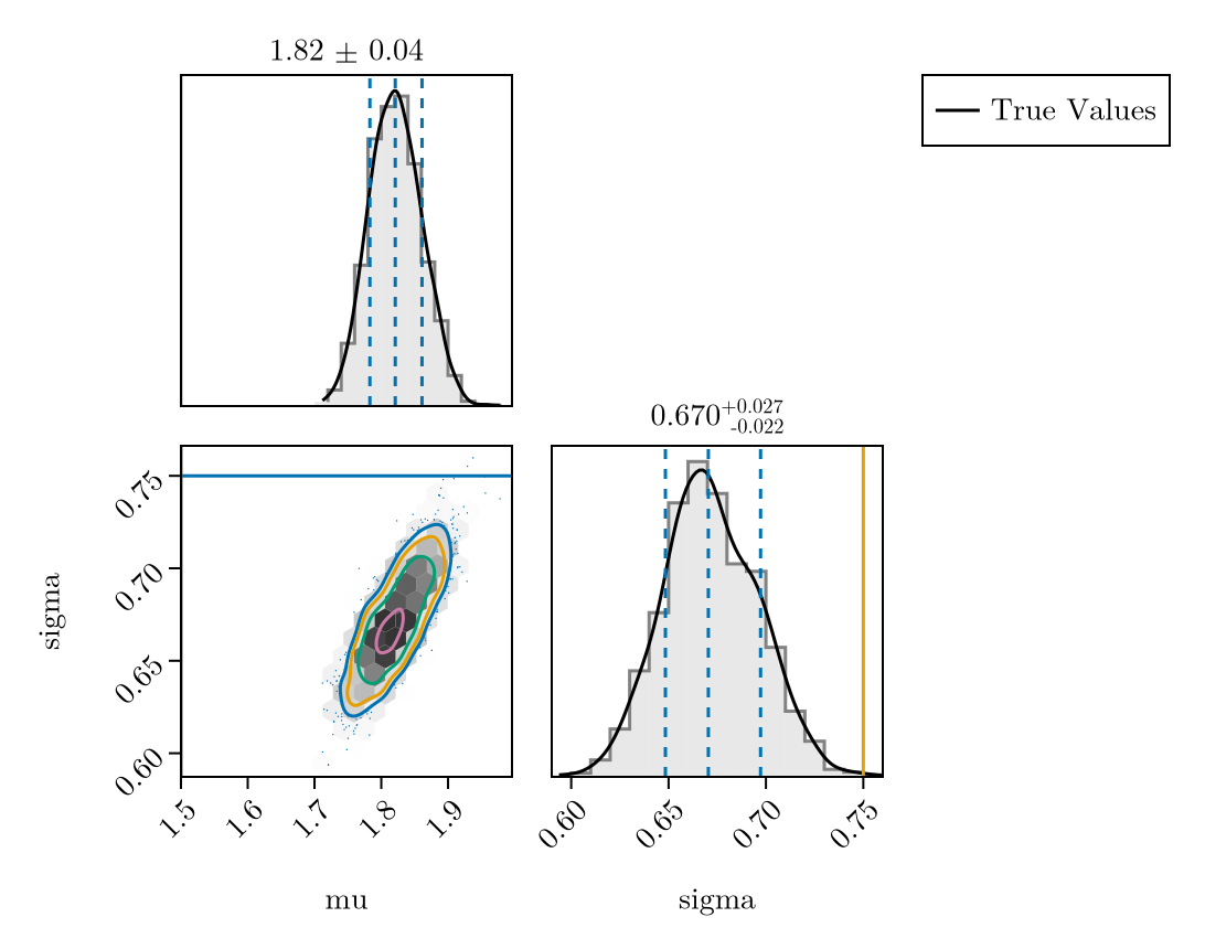
Lets plot the posterior compared to the true values again. *Note: An annoying feature to to_submodel() is that it automatically prefixes the LHS name to all variables names in the model meaning we need to customise our postprocessing or turn this feature off.

plot_fit_with_truth(interval_only_fit, Dict("dist.mu" => meanlog, "dist.sigma" => sdlog))

Fitting the full CensoredDistributions model

Now we'll fit the full model that accounts for the censoring process. Since the CensoredDistributions_model was defined earlier and used for simulation, we'll reuse it for fitting - demonstrating the consistency of our approach.

CensoredDistributions_mdl = @with simulated_counts begin
    CensoredDistributions_model(:observed_delay, :n, :primary_dist,
        :swindow, :obs_time)
end

Model{typeof(CensoredDistributions_model), (:y, :n, :primary_dists, :sws, :Ds), (), (), Tuple{Vector{Float64}, Vector{Int64}, Vector{Uniform{Float64}}, Vector{Int64}, Vector{Int64}}, Tuple{}, DefaultContext}(CensoredDistributions_model, (y = [8.0, 3.0, 5.0, 3.0, 8.0, 0.0, 3.0, 7.0, 4.0, 4.0  …  0.0, 0.0, 1.0, 9.0, 11.0, 11.0, 9.0, 0.0, 10.0, 0.0], n = [8, 24, 15, 13, 17, 4, 25, 8, 35, 15  …  1, 5, 2, 2, 1, 2, 2, 3, 3, 1], primary_dists = Uniform{Float64}[Distributions.Uniform{Float64}(a=0.0, b=2.0), Distributions.Uniform{Float64}(a=0.0, b=1.0), Distributions.Uniform{Float64}(a=0.0, b=2.0), Distributions.Uniform{Float64}(a=0.0, b=1.0), Distributions.Uniform{Float64}(a=0.0, b=2.0), Distributions.Uniform{Float64}(a=0.0, b=2.0), Distributions.Uniform{Float64}(a=0.0, b=2.0), Distributions.Uniform{Float64}(a=0.0, b=1.0), Distributions.Uniform{Float64}(a=0.0, b=1.0), Distributions.Uniform{Float64}(a=0.0, b=1.0)  …  Distributions.Uniform{Float64}(a=0.0, b=1.0), Distributions.Uniform{Float64}(a=0.0, b=1.0), Distributions.Uniform{Float64}(a=0.0, b=2.0), Distributions.Uniform{Float64}(a=0.0, b=2.0), Distributions.Uniform{Float64}(a=0.0, b=2.0), Distributions.Uniform{Float64}(a=0.0, b=1.0), Distributions.Uniform{Float64}(a=0.0, b=1.0), Distributions.Uniform{Float64}(a=0.0, b=2.0), Distributions.Uniform{Float64}(a=0.0, b=2.0), Distributions.Uniform{Float64}(a=0.0, b=2.0)], sws = [1, 1, 1, 1, 2, 2, 1, 1, 2, 1  …  1, 2, 1, 1, 1, 1, 1, 2, 1, 1], Ds = [11, 10, 8, 8, 10, 11, 8, 11, 10, 9  …  10, 9, 10, 10, 12, 12, 10, 10, 12, 10]), NamedTuple(), DefaultContext())

Now we fit the model to recover the true parameters from the synthetic data we generated earlier. This demonstrates the package's ability to perform accurate parameter recovery when the censoring process is properly modelled.

CensoredDistributions_fit = sample(
    CensoredDistributions_mdl, NUTS(), MCMCThreads(), 1000, 4);

summarize(CensoredDistributions_fit)

	parameters	mean	std	mcse	ess_bulk	ess_tail	rhat	ess_per_sec
1	Symbol("dist.mu")	1.4889	0.0315059	0.000803063	1571.78	1732.8	1.00189	56.4537
2	Symbol("dist.sigma")	0.729124	0.0250392	0.000645892	1519.19	1780.99	1.0003	54.5646

plot_fit_with_truth(
    CensoredDistributions_fit, Dict("dist.mu" => meanlog, "dist.sigma" => sdlog))

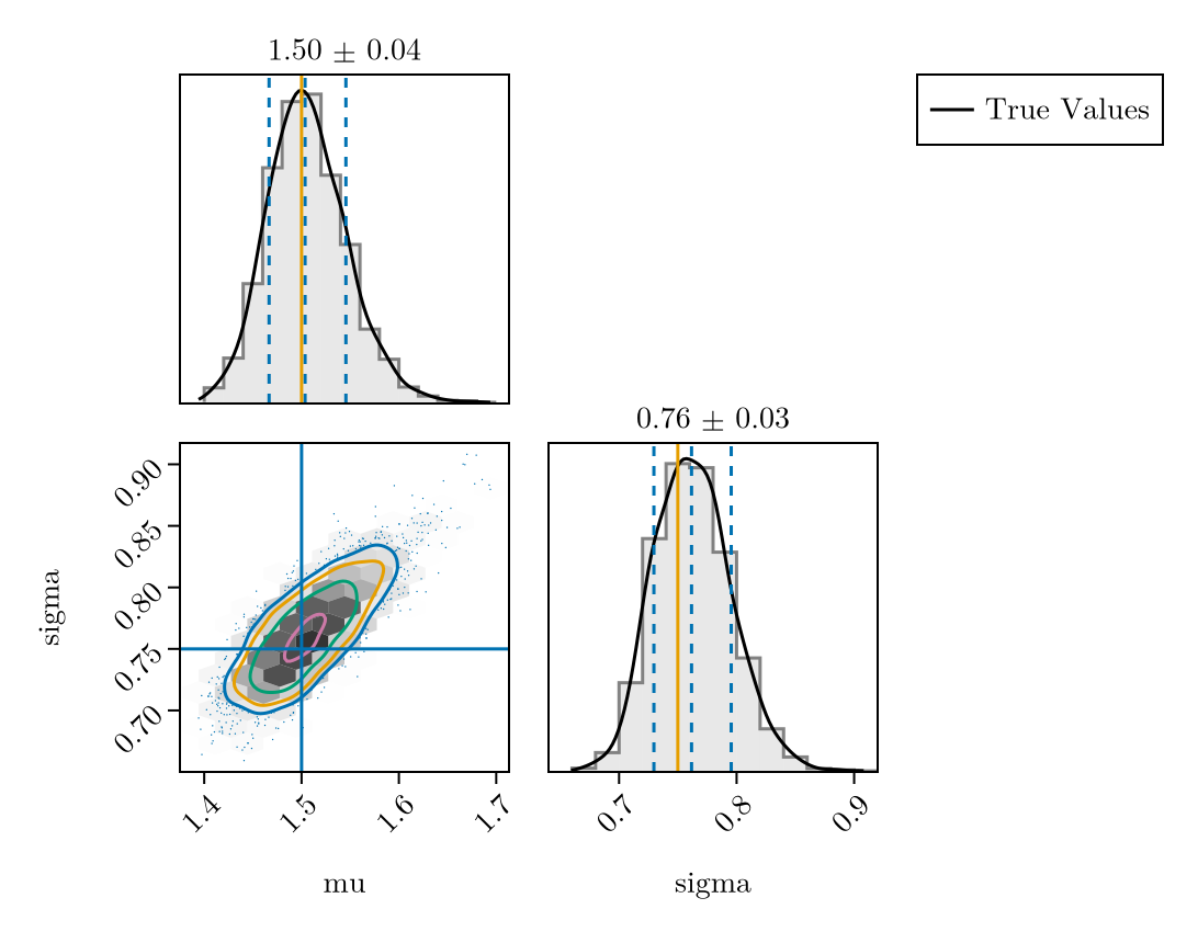
We see that the model has converged and the diagnostics look good. We also see that the posterior means are near the true parameters and the 90% credible intervals include the true parameters.