Automatic differentiation backends

CensoredDistributions.jl composes with Julia's automatic differentiation (AD) ecosystem, so the censored logpdf can be used as the likelihood in gradient-based inference, for example inside a Turing.jl model. This page reports which backends work, how to configure the ones that need it, and what each costs on the package's shared scenario set. Advice on choosing a backend and on debugging comes after the results.

Backend support

Each backend has its own AD gradient CI run, so a transiently unstable backend only reds its own badge. The badges below show the latest run of each on main, tested on Julia 1 (the latest stable release).

ForwardDiff	ReverseDiff (tape)	Enzyme forward	Enzyme reverse	Mooncake reverse	Mooncake forward

The top row is each backend's latest CI run: a green badge means that backend differentiates the scenarios we test for it, which does not by itself mean full coverage. The second row is each backend's code coverage from the gradient suite (Codecov flag ad-<backend>), reporting which package lines that backend exercises. All six backends (ForwardDiff, ReverseDiff (tape), Enzyme forward, Enzyme reverse, Mooncake reverse, Mooncake forward) cover the whole scenario set.

Configuring Enzyme

Enzyme needs one caller-side setting to work through the numerical (quadrature) paths.

using ADTypes, Enzyme
AutoEnzyme(mode = Enzyme.set_runtime_activity(Enzyme.Reverse))

set_runtime_activity defers per-value activity decisions to runtime; see the Enzyme FAQ for what it does. These are the settings the benchmark below uses. The observation data is passed as a Constant DifferentiationInterface context rather than captured in a closure, which keeps the differentiated function free of active fields. Runtime activity is not free. On the analytical paths, which do not need it, it makes Enzyme several times slower here, so its benchmark rows are conservative; the benchmark applies one Enzyme configuration to every scenario and only the numerical paths require it. Running through DifferentiationInterface, by contrast, adds no measurable overhead.

The scenario set covers analytical and numerical paths for Gamma, LogNormal, and Weibull delays with both Uniform and ExponentiallyTilted primary events, plus IntervalCensored and DoubleIntervalCensored constructions.

It spans two regimes so the comparison is not limited to the small fits that favour forward mode. Most scenarios are low-dimensional (two or three parameters), matching a single delay fit. A further set gives each observation its own delay parameter (32 in all), in analytical and numerical forms, to exercise the high-dimensional regime. The numerical (quadrature) paths also do much more work per call than the analytical ones, stressing how each backend differentiates the integration routine.

It is defined with DifferentiationInterfaceTest.jl in the ADFixtures path package at test/ADFixtures, and shared with the gradient tests (test/ad/runtests.jl) and the benchmark suite (benchmark/src/ad_gradients.jl).

Packages used

Show setup code

using CensoredDistributions
using Distributions
using ADTypes
using DifferentiationInterface
import DifferentiationInterfaceTest as DIT
using ForwardDiff
using ReverseDiff
using Enzyme
using Mooncake
using Chairmarks
using ADFixtures
using DataFramesMeta
using Statistics
using CairoMakie
using AlgebraOfGraphics

CairoMakie.activate!(type = "png", px_per_unit = 2)
set_theme!(theme_latexfonts(); fontsize = 14)

scenarios = ADFixtures.scenarios()
all_backends = [entry.backend for entry in ADFixtures.backends()]
backend_name = Dict(entry.backend => entry.name
for entry in ADFixtures.backends())

Dict{ADTypes.AbstractADType, String} with 6 entries:
  AutoReverseDiff()                                      => "ReverseDiff (tape)"
  AutoForwardDiff()                                      => "ForwardDiff"
  AutoMooncakeForward()                                  => "Mooncake forward"
  AutoMooncake()                                         => "Mooncake reverse"
  AutoEnzyme(mode=ForwardMode{false, FFIABI, false, tru… => "Enzyme forward"
  AutoEnzyme(mode=ReverseMode{false, true, false, FFIAB… => "Enzyme reverse"

Benchmark

DifferentiationInterfaceTest.benchmark_differentiation runs every (backend, scenario) pair. We pass every backend and scenario so broken combinations show up as gaps rather than being hidden. The figures are the prepared per-call cost. DifferentiationInterface prepares each backend once, recording a tape for ReverseDiff and compiling a rule for Enzyme and Mooncake, and we time the reused operator, so that one-off preparation is excluded. This matches repeated use such as an MCMC run, where preparation is amortised over many gradient calls. Each backend's time and allocations are then divided by the ForwardDiff value on the same scenario, so ForwardDiff sits at 1.0 by construction; values below 1.0 are faster (or lighter), above 1.0 slower (or heavier).

Summary

Geometric mean of the relative cost across the scenarios each backend can handle. Scenarios reports coverage, since a partial backend averages only over the scenarios it differentiates.

Show benchmark code

raw_bench = DIT.benchmark_differentiation(
    all_backends, scenarios;
    logging = false,
    benchmark_test = false
)

# `replace` order matters because `DoubleIntervalCensored` contains
# `IntervalCensored`; the longer key is matched first.
function _shorten(name)
    replace(name,
        "DoubleIntervalCensored" => "DIC",
        "IntervalCensored" => "IC",
        "PrimaryCensored" => "PC")
end

bench_long = @chain DataFrame(raw_bench) begin
    @rsubset :operator == ^(:gradient)
    @rtransform begin
        :backend = backend_name[:backend]
        :scenario = _shorten(:scenario.name)
        :time_us = :time * 1e6
        :bytes_kb = :bytes / 1024
    end
    @rsubset isfinite(:time_us) && isfinite(:bytes_kb)
    @select :backend :scenario :time_us :bytes_kb
end;

ref = @chain bench_long begin
    @rsubset :backend == "ForwardDiff"
    @select :scenario :ref_time=:time_us :ref_bytes=:bytes_kb
end

rel = @chain bench_long begin
    leftjoin(ref, on = :scenario)
    @rtransform begin
        :rel_time = :time_us / :ref_time
        :rel_bytes = :bytes_kb / :ref_bytes
    end
end;

# Geometric mean over positive values; guards against a zero-allocation
# scenario sending `log` to -Inf.
function geomean(x)
    pos = filter(>(0), x)
    isempty(pos) ? NaN : exp(mean(log.(pos)))
end

n_total = length(unique(bench_long.scenario))

summary = @chain rel begin
    @by :backend begin
        :rel_time = round(geomean(:rel_time); digits = 2)
        :rel_bytes = round(geomean(:rel_bytes); digits = 2)
        :scenarios = "$(length(:scenario))/$(n_total)"
    end
    @orderby :rel_time
    rename(
        :backend => "Backend",
        :rel_time => "Relative time",
        :rel_bytes => "Relative allocations",
        :scenarios => "Scenarios")
end;

Test Summary:                                                                                            | Total      Time
Testing benchmarks                                                                                       |     0  15m30.5s
  ADTypes.AutoForwardDiff()                                                                              |     0   1m47.5s
  ADTypes.AutoReverseDiff()                                                                              |     0   1m23.1s
  ADTypes.AutoMooncake()                                                                                 |     0   3m58.3s
  ADTypes.AutoMooncakeForward()                                                                          |     0   2m22.8s
  ADTypes.AutoEnzyme(mode=EnzymeCore.ReverseMode{false, true, false, EnzymeCore.FFIABI, false, false}()) |     0   3m48.3s
  ADTypes.AutoEnzyme(mode=EnzymeCore.ForwardMode{false, EnzymeCore.FFIABI, false, true, false}())        |     0   2m10.3s

summary

6×4 DataFrame

Row	Backend	Relative time	Relative allocations	Scenarios
	String	Float64	Float64	String
1	Enzyme forward	0.98	0.66	28/28
2	ForwardDiff	1.0	1.0	28/28
3	Mooncake reverse	1.3	0.28	28/28
4	Enzyme reverse	1.49	6.84	28/28
5	Mooncake forward	3.27	2.1	28/28
6	ReverseDiff (tape)	17.18	253.91	28/28

Spread across scenarios

Each box summarises a backend's relative cost across the scenario set, on a log scale so speed-ups and slow-downs are symmetric around the ForwardDiff baseline at 1.0.

Show plotting code

plot_df = @chain rel begin
    stack([:rel_time, :rel_bytes],
        variable_name = :metric, value_name = :value)
    @rsubset :value > 0
    @rtransform begin
        :metric = :metric == "rel_time" ? "Relative time" :
                  "Relative allocations"
        :family = startswith(:backend, "Enzyme") ? "Enzyme" :
                  startswith(:backend, "Mooncake") ? "Mooncake" :
                  startswith(:backend, "ReverseDiff") ? "ReverseDiff" :
                  "ForwardDiff"
        :mode = (occursin("reverse", :backend) ||
                 startswith(:backend, "ReverseDiff")) ? "reverse" :
                "forward"
    end
end

# Order the facets time-then-allocations.
metric_order = sorter(["Relative time", "Relative allocations"])

fig_relative = draw(
    data(plot_df) *
    mapping(
        :backend => "",
        :value => "Cost relative to ForwardDiff",
        col = :metric => metric_order) *
    visual(BoxPlot);
    figure = (size = (1200, 500),),
    axis = (yscale = log10, xticklabelrotation = pi / 4),
    facet = (; linkyaxes = :none)
);

fig_relative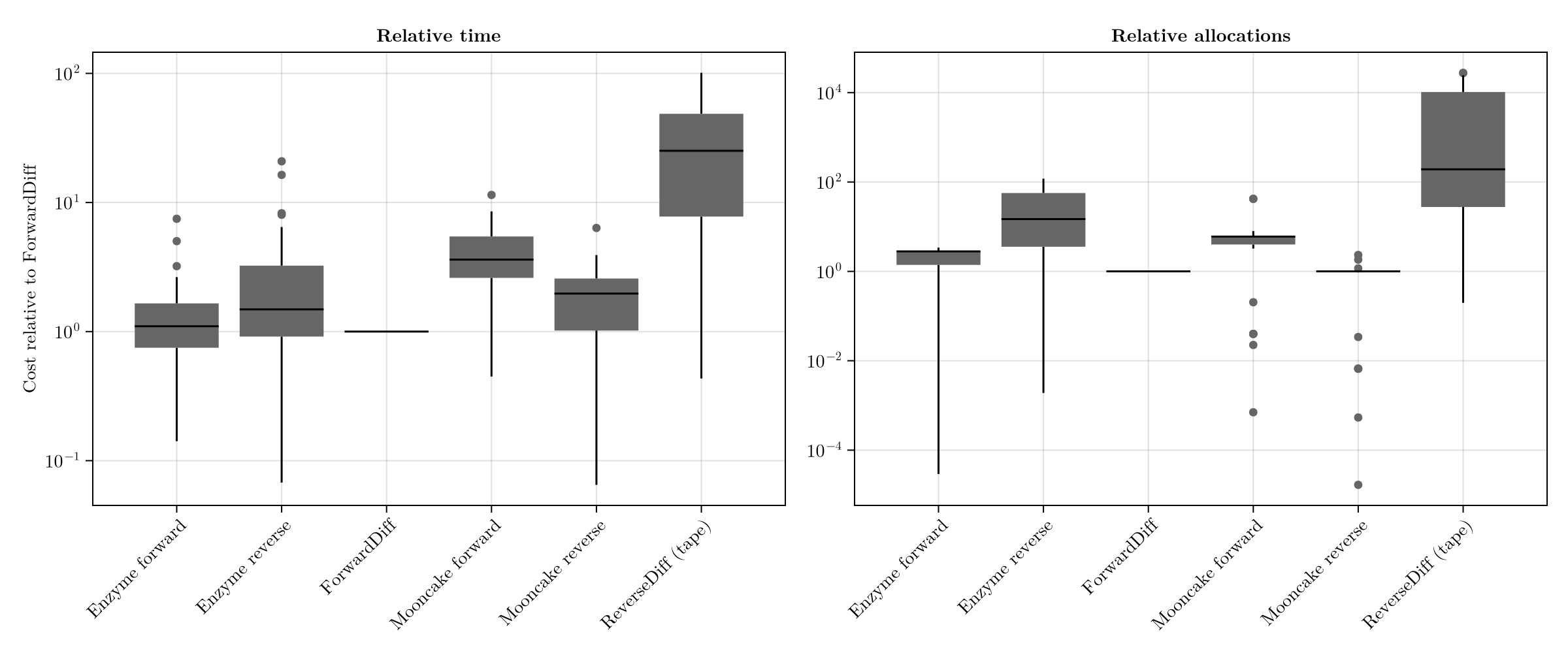

Per scenario

The same data with one point per scenario, so individual outliers show rather than being summarised. Scenarios on the horizontal axis, relative cost on the vertical axis (log scale), backends by colour, faceted by metric.

Show plotting code

fig_scenarios = draw(
    data(plot_df) *
    mapping(
        :scenario => "",
        :value => "Cost relative to ForwardDiff",
        color = :family => "Backend family",
        marker = :mode => "Mode",
        col = :metric => metric_order) *
    visual(Scatter, markersize = 11);
    figure = (size = (1600, 800),),
    axis = (yscale = log10, xticklabelrotation = pi / 4),
    facet = (; linkyaxes = :none)
);

fig_scenarios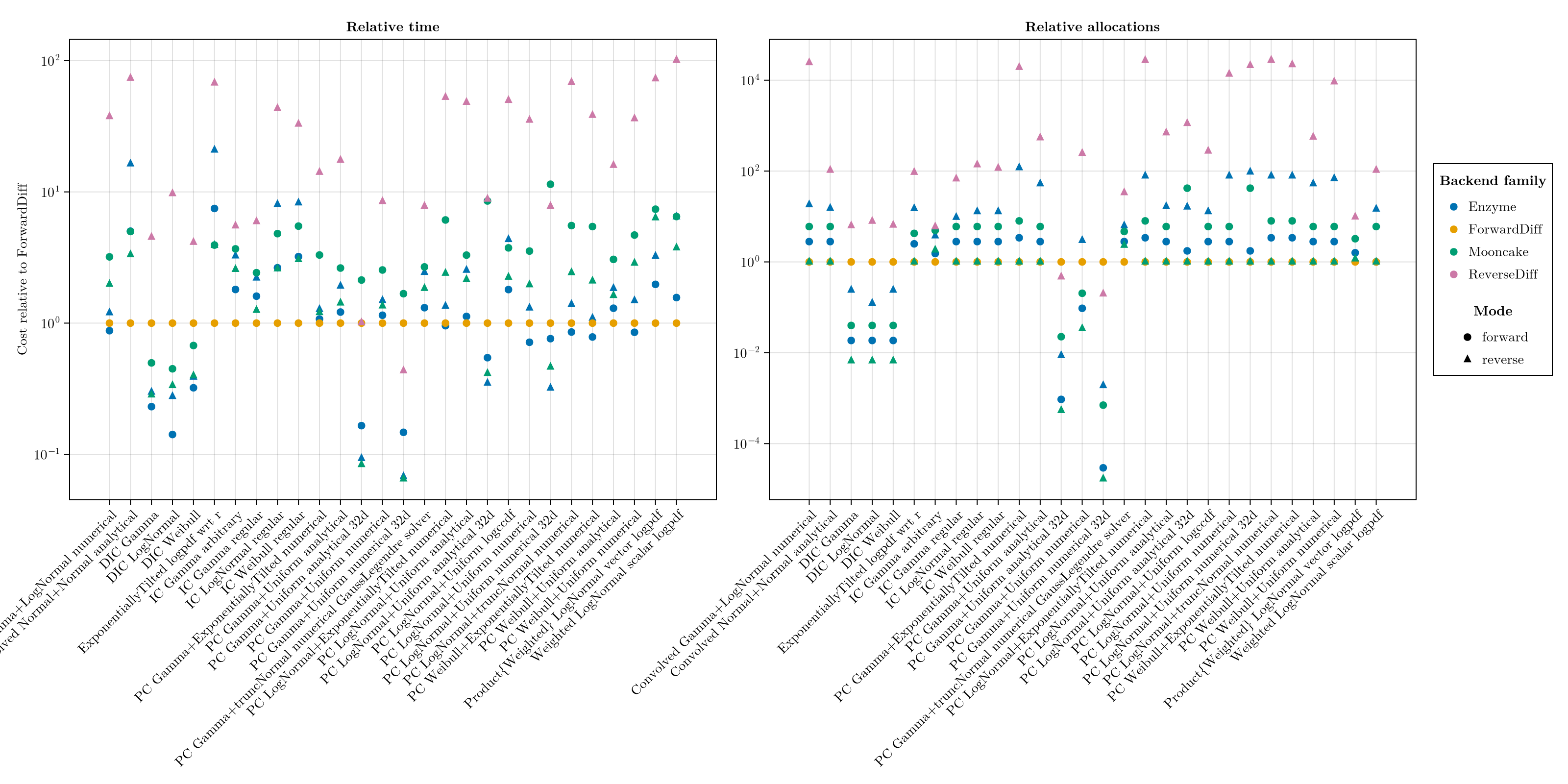

The full long-format result is available as raw_bench if you want GC fraction, compile fraction, the value_and_gradient rows, or absolute timings.

Choosing a backend

The results above reflect a general rule: which backend is fastest depends on how many parameters you differentiate with respect to.

• Forward mode (ForwardDiff, Enzyme forward, Mooncake forward) costs one pass per parameter, so it wins when the parameter count is small. Fitting a single censored delay distribution has two or three parameters, which is why ForwardDiff leads the low-dimensional rows. Among the forward backends ForwardDiff is fastest on these small smooth logpdfs; Enzyme and Mooncake forward do not beat it here.

• Reverse mode (ReverseDiff, Enzyme reverse, Mooncake reverse) costs one pass per output regardless of the parameter count, so it pays off once a censored distribution sits inside a larger model with many latent parameters. In the 32-parameter rows Enzyme reverse and Mooncake reverse run several times faster than ForwardDiff; ReverseDiff's tape overhead leaves it slower even there.

Turing's AD guidance puts the crossover around 20 parameters: forward mode below, reverse mode above. ForwardDiff is the simplest fast default for the small-parameter case and needs no configuration. For a higher-dimensional model, switch to a reverse-mode backend; Enzyme and Mooncake show their strength here, in reverse rather than forward mode. In a Turing model you set this through the sampler's adtype, for example sample(model, NUTS(; adtype = AutoMooncake()), 1000), and the surest choice is to benchmark the backends on your own model.

Debugging

ForwardDiff fails with ordinary Julia MethodErrors that point at the offending call, so it is the easiest backend to debug; start there when a gradient misbehaves. Enzyme and Mooncake report errors at the compiled-IR level, which are harder to trace.

DifferentiationInterface and DifferentiationInterfaceTest make this tractable. DI gives one gradient call that swaps backends without touching the model, so you can compare a suspect backend against the ForwardDiff value on the same input (which is what the gradient tests do). DIT runs a single function across several backends at once and flags the ones that disagree with the reference. Work bottom-up: differentiate one small piece first (a single logpdf, then a primary_censored logpdf), confirm it, and build up to the full model, so the construct a backend chokes on is easy to isolate.

Reproducing this page

The numbers above are measured on the docs-build machine, so they reflect that CPU. To regenerate locally:

task docs

or, equivalently:

julia --project=docs docs/make.jl

See also

• test/ad/ holds the gradient tests as tagged @testitems, validated against a ForwardDiff reference with DifferentiationInterfaceTest.test_differentiation. Pass a backend tag (e.g. TAG=enzyme_reverse task test-ad-backend) to run a single backend, as the per-backend CI does.

• benchmark/src/ad_gradients.jl runs the same scenarios under AirspeedVelocity. A benchmark history timeline is tracked in #224.